Example of full workflow • RRatepol

This workflow should show the full strength of the RRatepol package and serve as step-by-step guidance starting from downloading dataset from Neotoma, building age-depth models, to estimating rate-of-change using age uncertainty.

⚠️This workflow is only meant as an example: There are several additional steps for data preparation, which should be done to properly implement RRatepol and assess the rate of change of a fossil pollen dataset from Neotoma!

For an even more detailed step-by-step workflow with fossil pollen data, please see other package materials, such as African Polled Database workshop.

Additionally, please see FOSSILPOL, an R-based modular workflow to process multiple fossil pollen records to create a comprehensive, standardized dataset compilation, ready for multi-record and multi-proxy analyses at various spatial and temporal scales.

Finally, for workflows using other data types (e.g., geochemistry and XRF), see Oeschger Centre for Climate Change Research Workshop.

Install packages

Make a list of packages needed from CRAN

package_list <-
  c(
    "tidyverse", # general data wrangling and visualisation
    "neotoma2", # access to the Neotoma database
    "pander", # nice tables
    "Bchron", # age-depth modelling
    "janitor", # string cleaning
    "remotes" # installing packages from GitHub
  )

Install all packages from CRAN

lapply(
  package_list, utils::install.packages
)

Attach packages

library(tidyverse) # general data wrangling and visualisation
library(pander) # nice tables
library(RRatepol) # rate-of-vegetation change
library(neotoma2) # obtain data from the Neotoma database
library(Bchron) # age-depth modeling
library(janitor) # string cleaning

Download the dataset Glendalough Valley from Neotoma

gl_dataset_download <-
  neotoma2::get_downloads(17334)

Prepare the pollen counts

# get samples
gl_counts <-
  neotoma2::samples(gl_dataset_download)

# select only "pollen" taxa
gl_taxon_list_selected <-
  neotoma2::taxa(gl_dataset_download) %>%
  dplyr::filter(element == "pollen") %>%
  purrr::pluck("variablename")

# prepare taxa table
gl_counts_selected <-
  gl_counts %>%
  as.data.frame() %>%
  dplyr::mutate(sample_id = as.character(sampleid)) %>%
  tibble::as_tibble() %>%
  dplyr::select("sample_id", "value", "variablename") %>%
  # only include selected taxons
  dplyr::filter(
    variablename %in% gl_taxon_list_selected
  ) %>%
  # turn into the wider format
  tidyr::pivot_wider(
    names_from = "variablename",
    values_from = "value",
    values_fill = 0
  ) %>%
  # clean names
  janitor::clean_names()

head(gl_counts_selected)[, 1:5]

sample_id	larix	cichorioideae	prunus_type	apiaceae
161508	1	1	1	1
161509	0	1	0	0
161510	0	1	0	0
161511	0	1	0	0
161512	0	2	0	0
161513	0	0	0	1

Here, we strongly advocate that attention should be paid to the selection of the ecological groups as well as the harmonisation of the pollen taxa. However, that is not the subject of this workflow, but any analysis to be published needs careful preparation of the fossil pollen datasets before using R-Ratepol!

Preparation of the levels

Sample depth

Extract depth for each level

gl_level <-
  neotoma2::samples(gl_dataset_download) %>%
  tibble::as_tibble() %>%
  dplyr::mutate(sample_id = as.character(sampleid)) %>%
  dplyr::distinct(sample_id, depth) %>%
  dplyr::relocate(sample_id)

head(gl_level)

sample_id	depth
161508	0
161509	8
161510	16
161511	24
161512	32
161513	40

Age depth modelling

e will recalculate the age-depth model ‘de novo’ using the Bchron package.

Prepare chron.control table and run Bchron

The chronology control table contains all the dates (mostly radiocarbon) to create the age-depth model.

Here we only present a few of the important steps of preparation of the chronology control table. There are many more potential issues, but solving those is not the focus of this workflow.

# First, get the chronologies and check which we want to use used
gl_chron_control_table_download <-
  neotoma2::chroncontrols(gl_dataset_download)

print(gl_chron_control_table_download)

Table continues below
siteid	chronologyid	depth	thickness	agelimitolder	chroncontrolid
11577	9691	0	0	-45	37155
11577	9691	210	3	1710	37156
11577	9691	426	4	2340	37157
11577	9691	630	4	2530	37158
11577	9691	1056	3	4090	37159
11577	9691	1105	4	4510	37160

agelimityounger	chroncontrolage	chroncontroltype
-45	-45	Core top
1590	1650	Radiocarbon
2280	2310	Radiocarbon
2470	2500	Radiocarbon
4030	4060	Radiocarbon
4410	4460	Radiocarbon

# prepare the table
gl_chron_control_table <-
  gl_chron_control_table_download %>%
  dplyr::filter(chronologyid == 9691) %>%
  tibble::as_tibble() %>%
  # Here we calculate the error as the average of the age `limitolder` and
  #   `agelimityounger`
  dplyr::mutate(
    error = round((agelimitolder - agelimityounger) / 2)
  ) %>%
  # As Bchron cannot accept a error of 0, we need to replace the value with 1
  dplyr::mutate(
    error = replace(error, error == 0, 1),
    error = ifelse(is.na(error), 1, error)
  ) %>%
  # We need to specify which calibration curve should be used for what point
  dplyr::mutate(
    curve = ifelse(as.data.frame(gl_dataset_download)["lat"] > 0, "intcal20", "shcal20"),
    curve = ifelse(chroncontroltype != "Radiocarbon", "normal", curve)
  ) %>%
  tibble::column_to_rownames("chroncontrolid") %>%
  dplyr::select(
    chroncontrolage, error, depth, thickness, chroncontroltype, curve
  )

head(gl_chron_control_table)

Table continues below
	chroncontrolage	error	depth	thickness	chroncontroltype
37155	-45	1	0	0	Core top
37156	1650	60	210	3	Radiocarbon
37157	2310	30	426	4	Radiocarbon
37158	2500	30	630	4	Radiocarbon
37159	4060	30	1056	3	Radiocarbon
37160	4460	50	1105	4	Radiocarbon

	curve
37155	normal
37156	intcal20
37157	intcal20
37158	intcal20
37159	intcal20
37160	intcal20

As this is just a toy example, we will use only the iteration multiplier (i_multiplier) of 0.1 to reduce the computation time. However, we strongly recommend increasing it to 5 for any normal age-depth model construction.

i_multiplier <- 0.1 # increase to 5

# Those are default values suggested by the Bchron package
n_iteration_default <- 10e3
n_burn_default <- 2e3
n_thin_default <- 8

# Let's multiply them by our i_multiplier
n_iteration <- n_iteration_default * i_multiplier
n_burn <- n_burn_default * i_multiplier
n_thin <- max(c(1, n_thin_default * i_multiplier))

gl_bchron <-
  Bchron::Bchronology(
    ages = gl_chron_control_table$chroncontrolage,
    ageSds = gl_chron_control_table$error,
    positions = gl_chron_control_table$depth,
    calCurves = gl_chron_control_table$curve,
    positionThicknesses = gl_chron_control_table$thickness,
    iterations = n_iteration,
    burn = n_burn,
    thin = n_thin
  )

Visually check the age-depth models

plot(gl_bchron)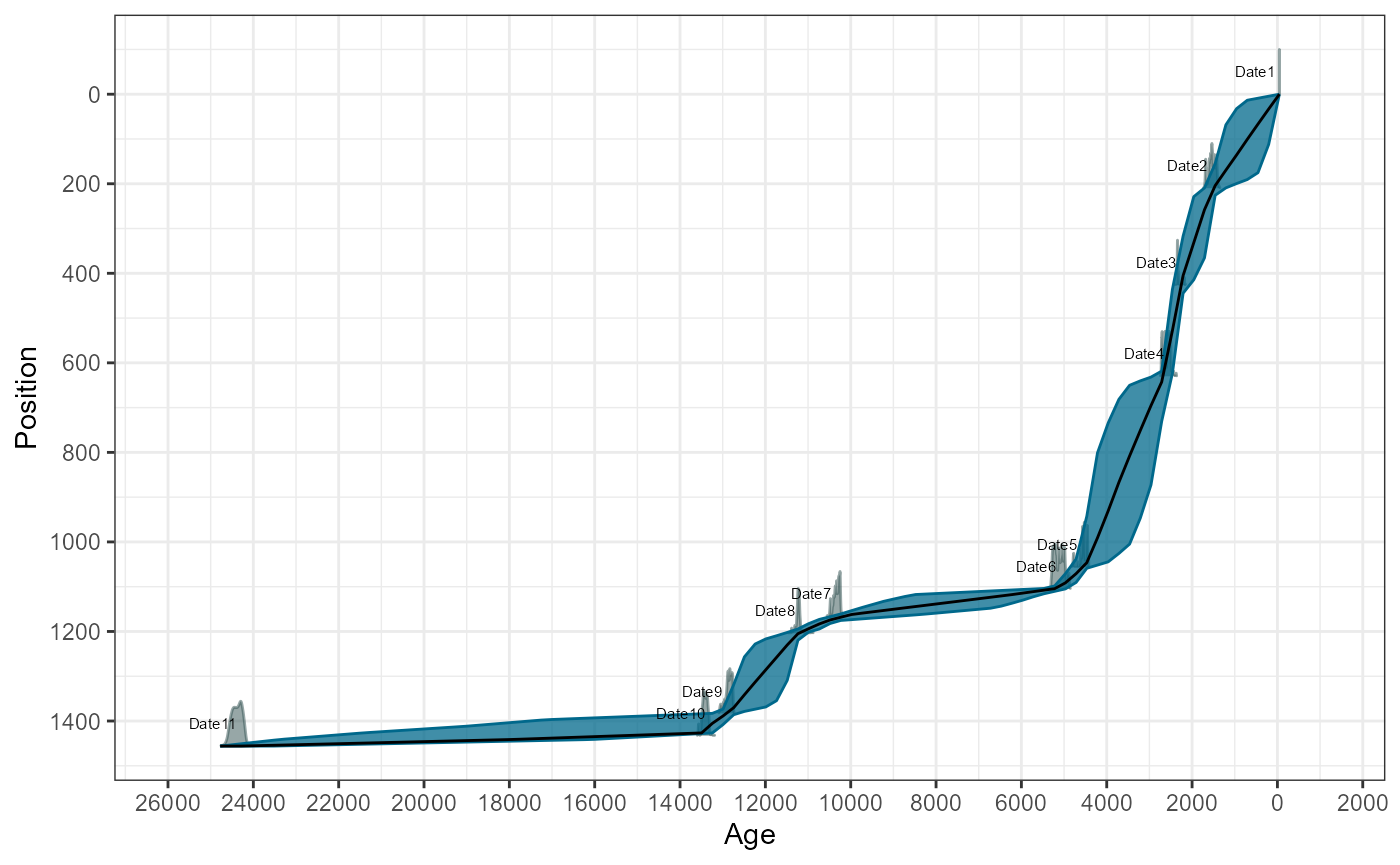

Predict ages

Let’s first extract posterior ages from the age-depth model (i.e. possible ages)

age_position <-
  Bchron:::predict.BchronologyRun(object = gl_bchron, newPositions = gl_level$depth)

age_uncertainties <-
  age_position %>%
  as.data.frame() %>%
  dplyr::mutate_all(., as.integer) %>%
  as.matrix()

colnames(age_uncertainties) <- gl_level$sample_id

gl_level_predicted <-
  gl_level %>%
  dplyr::mutate(
    age = apply(
      age_uncertainties, 2,
      stats::quantile,
      probs = 0.5
    )
  )

head(gl_level_predicted)

sample_id	depth	age
161508	0	-44
161509	8	16
161510	16	77
161511	24	138
161512	32	199
161513	40	259

Estimation Rate-of-Change

Here we use the the prepared data to estimate the rate of vegetation change. We will be using the Chi-squared coefficient as the dissimilarity coefficient (works best for pollen data, dissimilarity_coefficient = "chisq"), and time_standardisation == 500 (this means that all ROC values are ‘change per 500 yr’). We will add smoothing of the pollen data using smooth_method = "shep" (i.e. Shepard’s 5-term filter). Finally, we will use the method of the “binning with the mowing window” (working_units = "MW"). This is again a toy example for a quick computation and we would recommend increasing the set_randomisations to 10.000 for any real estimation.

set_randomisations <- 100 # increase to 10e3

gl_roc <-
  RRatepol::estimate_roc(
    data_source_community = gl_counts_selected,
    data_source_age = gl_level_predicted,
    age_uncertainty = age_uncertainties, # Add the uncertainty matrix
    smooth_method = "shep", # Shepard's 5-term filter
    dissimilarity_coefficient = "chisq",
    working_units = "MW", # set to "MW" to apply the "moving window"
    bin_size = 500, # size of a time bin
    number_of_shifts = 5,
    standardise = TRUE, # set the taxa standardisation
    n_individuals = 150, # set the number of pollen grains
    rand = set_randomisations, # set number of randomisations
    use_parallel = FALSE # use_parallel = TRUE to use parallel calculation
  )

Detect peak-points and plot the results

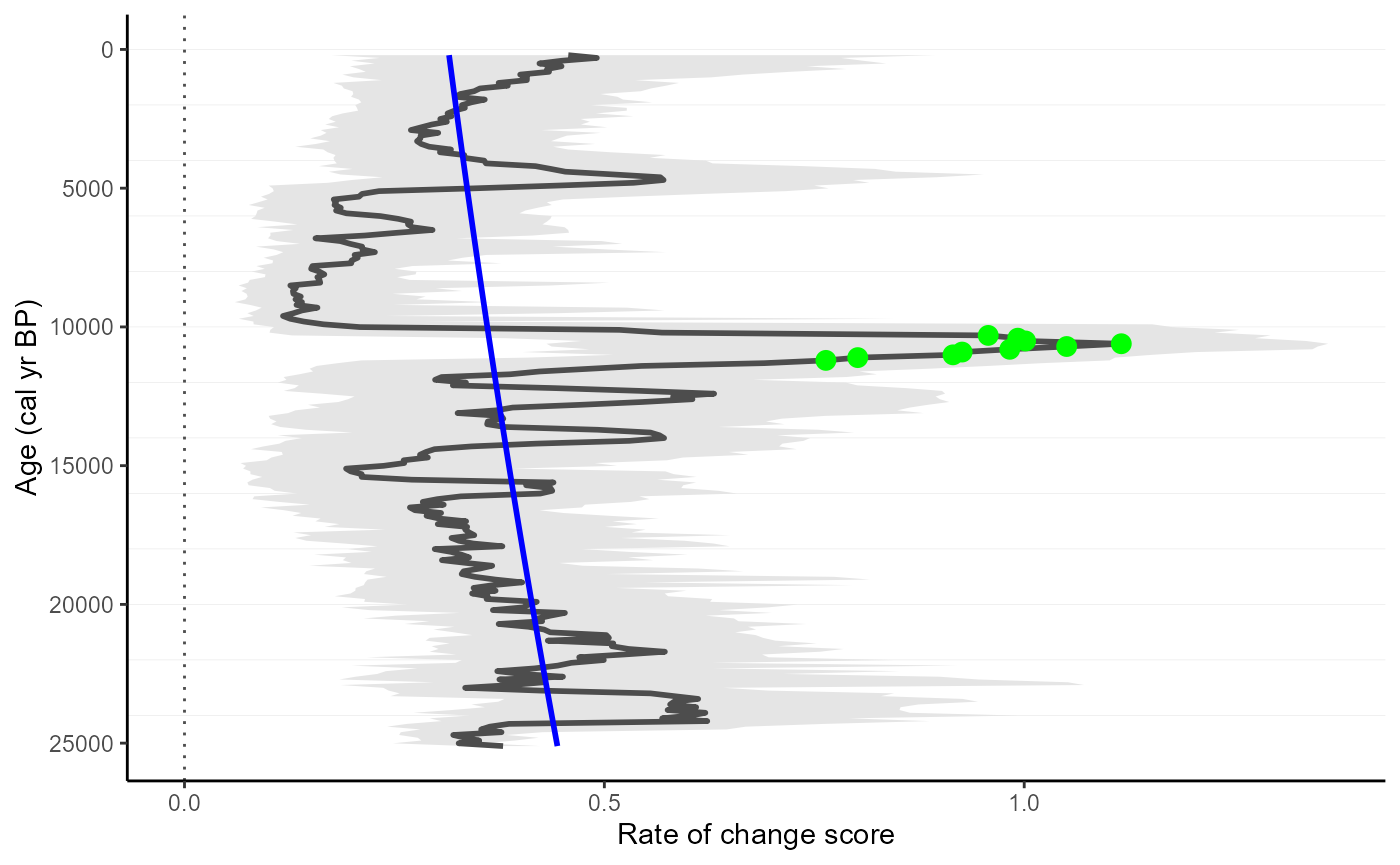
We will detect a significant increase in RoC values (i.e. peak-points). Specifically, we will use the “Non-linear” method, which will detect significant change from a non-linear trend of RoC

gl_roc_peaks <-
  RRatepol::detect_peak_points(
    data_source = gl_roc,
    sel_method = "trend_non_linear"
  )

Plot the estimates showing the peak-points

RRatepol::plot_roc(
  data_source = gl_roc_peaks,
  peaks = TRUE,
  trend = "trend_non_linear"
)