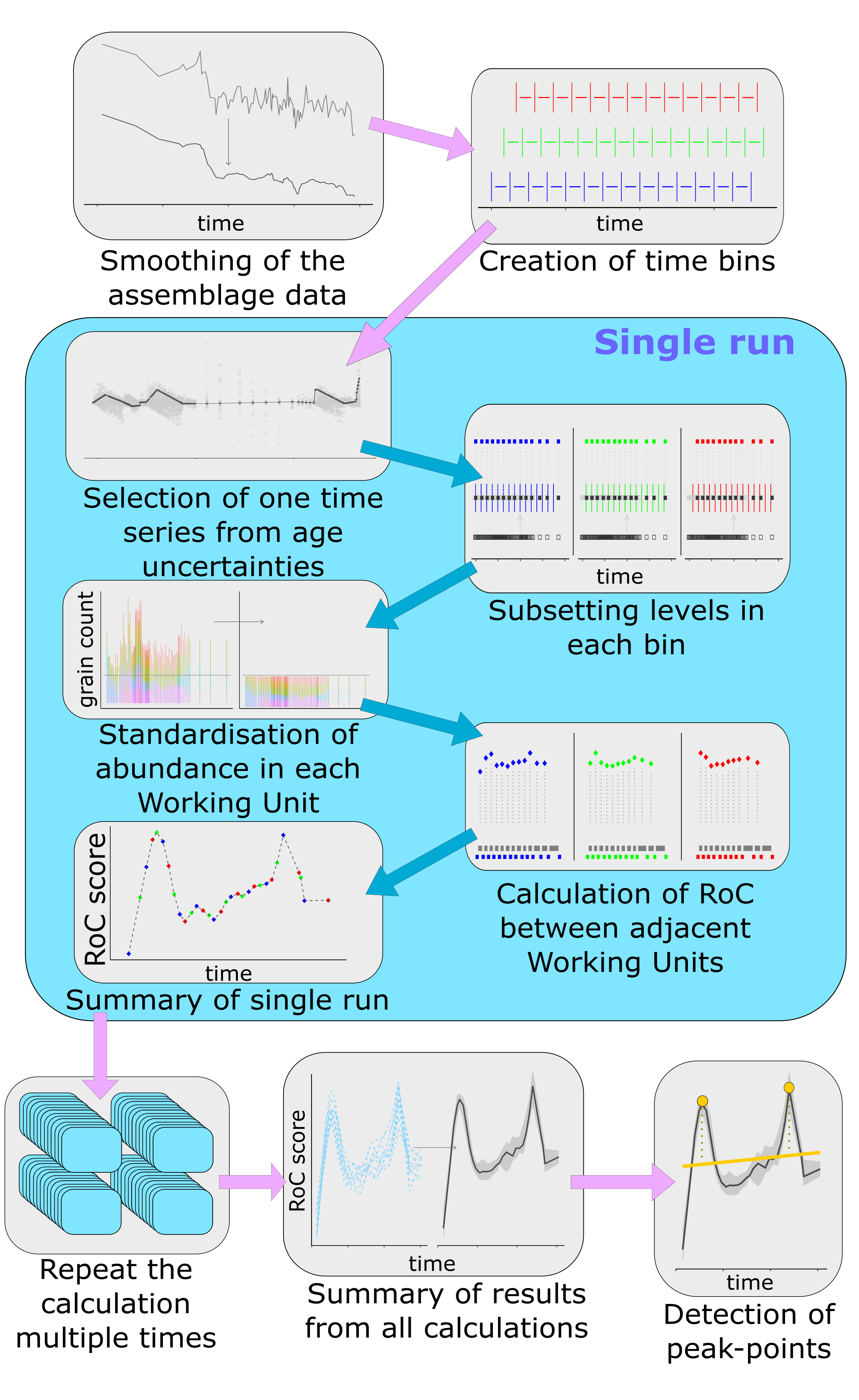
General RRatepol package description

Overview

RRatepol estimates the Rate of Change (RoC) in community composition along a temporal sequence. RoC is defined as the dissimilarity between consecutive assemblage samples, standardised by the time elapsed between them. The package is primarily designed for paleoecological data — such as fossil pollen records — but can be applied to any community dataset with a temporal axis.

The main function, estimate_roc(), accepts community counts and sample ages as inputs and returns a time series of RoC values. An optional second step, detect_peak_points(), identifies statistically significant peaks in that time series. Results can be visualised with plot_roc().

Input data

Two data frames are required:

Community data (data_source_community): samples as rows, taxa as columns, with the first column named sample_id.
Age data (data_source_age): two columns — sample_id and age (in years before present, or any consistent temporal unit).

An optional age-uncertainty matrix (age_uncertainty) can also be supplied. Each column represents one sample and each row a plausible age estimate drawn from a posterior age-depth model (e.g. from Bchron or Bacon). When provided, RRatepol uses this matrix to propagate age-model uncertainty through the RoC estimates (see Randomisation).

Smoothing

Before RoC is computed, each taxon can optionally be smoothed along the temporal axis to reduce short-term noise. Five methods are available via the smooth_method argument of estimate_roc():

`smooth_method`	Description
`"none"`	No smoothing (default)
`"shep"`	Shepard’s 5-term filter (Davis, 1986; Wilkinson, 2005)
`"m.avg"`	Moving average
`"age.w"`	Age-weighted average
`"grim"`	Grimm’s smoothing (Grimm & Jacobson, 1992)

For "m.avg", "grim", and "age.w", the window is controlled by smooth_n_points (number of samples; must be odd) and smooth_age_range (maximum age span of the window). For "shep", smooth_n_points sets the number of points used in the polynomial fit.

Working units

RoC is calculated between consecutive Working Units (WUs). The definition of WUs is the most consequential methodological choice in an analysis. Three strategies are available via the working_units argument.

Individual levels (`"levels"`)

Each stratigraphical level is its own WU. This preserves maximum resolution but makes RoC values sensitive to uneven sampling density — closely spaced samples will produce smaller RoC values simply because less time elapsed between them.

Selective binning (`"bins"`)

Levels are grouped into time bins of width bin_size (years). One representative level is selected per bin, either at random (bin_selection = "random") or as the first level in the bin (bin_selection = "first"). Assemblage data are not pooled. This reduces sensitivity to uneven temporal spacing at the cost of resolution.

Moving-window binning (`"MW"`) — recommended

Moving-window binning extends selective binning by repeating the selection step with the bin window shifted forward by a fraction of bin_size. The shift amount is bin_size / number_of_shifts. This creates number_of_shifts overlapping sets of WUs, all of which are retained and summarised together.

This approach reduces the sensitivity of selective binning to the arbitrary placement of bin boundaries, while retaining its resistance to uneven sampling density. It is the recommended strategy for most analyses.

Diagram showing level, bin, and moving-window working-unit strategies — Schematic overview of working-unit strategies in RRatepol.

Dissimilarity coefficients

RoC between two consecutive WUs is defined as:

$\text{RoC} = \frac{D(WU_i,\ WU_{i+1})}{\Delta t}$

where $D$ is a dissimilarity coefficient and $\Delta t$ is the age difference between the two WUs. The choice of coefficient should match the properties of the assemblage data. Six coefficients are available via the dissimilarity_coefficient argument:

`dissimilarity_coefficient`	Description
`"euc"`	Euclidean distance
`"euc.sd"`	Standardised Euclidean distance
`"chord"`	Chord distance
`"chisq"`	Chi-squared coefficient
`"gower"`	Gower’s distance
`"bray"`	Bray-Curtis dissimilarity

See vegan::vegdist() for detailed definitions. For percentage-based data such as pollen, Chord distance or Chi-squared are typically preferred.

By default $\Delta t$ equals bin_size. To standardise RoC values to a different time unit (e.g. per 100 years instead of per 500 years), set time_standardisation explicitly.

Assemblage data are converted to proportions before dissimilarity is computed by default (tranform_to_proportions = TRUE).

Randomisation

Because both age estimates and assemblage counts carry statistical uncertainty, estimate_roc() can be run many times (rand) and results summarised across runs (Birks & Gordon, 1985). Two sources of uncertainty can be propagated independently or together.

Age-model uncertainty

When age_uncertainty is supplied, each run draws one row at random from the matrix to use as the age sequence for that iteration. WU pairs therefore have slightly different time positions and $\Delta t$ values across runs. The final RoC value for each WU pair is reported as the median across all runs; the 95th quantile is reported as an upper uncertainty bound.

Assemblage standardisation

When standardise = TRUE, assemblage counts in each WU are rarefied to n_individuals before dissimilarity is computed. Random sampling without replacement draws the specified number of individuals from each WU (e.g. n_individuals = 150 pollen grains). This removes the influence of total count size on dissimilarity estimates and is especially important when count sizes vary substantially across samples.

Peak-point detection

After RoC has been estimated, detect_peak_points() identifies statistically significant increases in RoC values — intervals where the rate of compositional change was unusually rapid. A rapid change in composition or relative abundances can serve as a marker for comparing records and interpreting the potential drivers of assemblage change. Five detection methods are available via the sel_method argument:

Threshold (sel_method = "threshold"): Each point is compared to the median of the whole RoC sequence. A point is significant if its 95th-quantile RoC value (across randomisations) exceeds that global median.
Linear trend (sel_method = "trend_linear"): A linear model is fitted to RoC vs. age. A point is significant if its residual exceeds the mean by more than sd_threshold standard deviations (default sd_threshold = 2).
Non-linear trend (sel_method = "trend_non_linear"): A conservative GAM is fitted to RoC vs. age (RoC ~ s(age, k = 3); Wood, 2011). Residuals are used in the same way as for the linear trend, with the same sd_threshold.
F-deriv GAM (sel_method = "GAM_deriv"): A smooth GAM is fitted to RoC vs. age (RoC ~ s(age)). The first derivative and its simultaneous confidence intervals are estimated using the gratia package (Simpson, 2018). A point is significant if the confidence interval of the first derivative at that point excludes zero.
Signal-to-noise index (sel_method = "SNI"): The SNI approach of Kelly et al. (2011), originally developed for sediment-charcoal records, is applied to the RoC sequence. A point is significant if its SNI value exceeds 3.

References

Birks, H.J.B., Gordon, A.D., 1985. Numerical Methods in Quaternary Pollen Analysis. Academic Press, London.

Davis, J.C., 1986. Statistics and Data Analysis in Geology, 2nd edn. J. Wiley & Sons, New York.

Grimm, E.C., Jacobson, G.L., 1992. Fossil-pollen evidence for abrupt climate changes during the past 18000 years in eastern North America. Clim. Dyn. 6, 179–184.

Kelly, R.F., Higuera, P.E., Barrett, C.M., Feng Sheng, H., 2011. A signal-to-noise index to quantify the potential for peak detection in sediment-charcoal records. Quat. Res. 75, 11–17. https://doi.org/10.1016/j.yqres.2010.07.011

Simpson, G.L., 2018. Modelling palaeoecological time series using generalised additive models. Front. Ecol. Evol. 6, 1–21. https://doi.org/10.3389/fevo.2018.00149

Wilkinson, L., 2005. The Grammar of Graphics. Springer-Verlag, New York. https://doi.org/10.2307/2669493

Wood, S.N., 2011. Fast stable restricted maximum likelihood and marginal likelihood estimation of semiparametric generalized linear models. J. R. Stat. Soc. Ser. B Stat. Methodol. 73, 3–36.